MoodSwing Trading: Sentiment‑Driven Trading Signals (LLM‑enhanced)

MoodSwing Trading is my attempt to make “trade the news as it lands” real: a production‑minded platform that ingests headlines in near‑real time, scores their tone, blends the signal into a market‑readable index, and publishes probabilistic forecasts—exposed as both a dashboard and an open API. The core sell is accuracy: modern LLMs and recent NLP advances let the system read context (negation, sarcasm, entity roles, forward‑looking guidance) that lexicons miss, then fold that understanding into a calibrated, auditable signal. It began life as a lightweight Market Sentimentaliser; the current system is its hardened successor with explicit calibration, reproducible weighting, transparent versioning, and a UI/strategy contract you can trust. The narrative is simple: capture meaning faithfully, quantify it consistently, deliver it fast.

Why build this?

I wanted to test a tight hypothesis end‑to‑end: does fresh, context‑aware sentiment move fast markets in a measurable way—and can we capture it with sufficient fidelity to trade on it? Most “sentiment” widgets are hand‑wavy; I wanted every step—from raw text to MoodScore to μ/σ forecasts—to be explicit and replayable. If a value changed, I wanted to see why: which pieces of text moved the number, what the model understood about actors and events, which weights, what decay, and how that propagated into forecasts. I also wanted parity between the notebook and the dashboard: the same shapes, the same equations, the same parameters.

System at 10,000 ft

• APIs & services: Async FastAPI on Uvicorn/uvloop, Dockerised. REST for history/snapshots; WebSockets for live tape and sentiment; pydantic models for schema discipline; Problem‑Details for errors.
• Storage: PostgreSQL 15 (LIST‑partitioned by ticker/date) for articles, intraday & daily sentiment, and predictions; Redis for hot caches/pub‑sub fan‑out; S3 for raw‑text archival/backfills.
• Workers: Celery/Redis for ingestion, scoring, and forecast runs; idempotent jobs with keys; exponential backoff + jitter on transient errors; cron/Beat for SLAs.
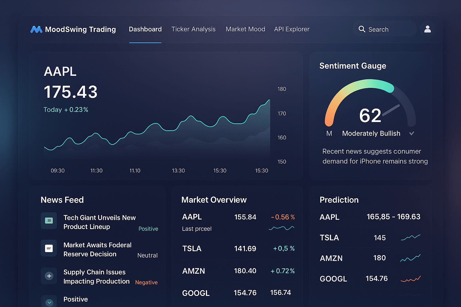
• Front‑end: React dashboard with live candlesticks, a MoodScore gauge (0–100) plus confidence ring, prediction cards with μ/σ, and ranked headline contributions.

From headline → signal → forecast

1) Ingest & normalise

On a minute cadence (configurable), the system pulls the last 60 minutes of headlines per ticker from upstream feeds. URLs are canonicalised (UTMs stripped, redirects resolved), language is detected, and soft‑duplicates are collapsed via shingling + simhash. Records are stored as:

article(ticker, provider, published_at, title, body, url_hash, url, s_i, p_i, r_i, model_version)

where s_i is filled below and model_version stamps the scoring build for auditability.

2) Per‑article sentiment (LLM‑first, ensembled & calibrated)

This is the accuracy upgrade.

• LLM layer (instruction‑tuned): A small service performs zero/few‑shot entity‑aware sentiment on the article→ticker relation, detects event type (earnings beat/miss, guidance change, litigation, M&A), and returns:

  • s_llm ∈ [−1,1] (polarity for the specific ticker),
  • conf_llm ∈ [0,1] (self‑reported confidence),
  • short rationale spans (text snippets) used as UI evidence,
  • optional structured tags (event=earnings_guidance_up, source=press_release, etc.). To keep latency workable, the service batches requests, caches by url_hash×ticker, and falls back to a distilled model when saturated. Mixed‑precision inference + ONNX runtime are used when available.

• Baselines for stability: NLTK VADER (robust on short headlines) and FinBERT (finance domain polarity) still run; spaCy provides NER/keyphrase spans to weight ticker‑proximal text.

• Ensemble & calibration: a linear/isotonic calibrator aligns outputs to a common score and learns mixture weights with optional confidence gating:

Outliers are winsorised (1st/99th pct) within a rolling window so single headlines cannot dominate aggregates. Why LLMs help: They parse things like “misses on EPS, raises FY guidance” (mixed signal), disambiguate who did what to whom, and handle negation/hedging (“not expected to impact”, “no material effect”)—classic failure modes for lexicons.

3) Impact weighting (recency × popularity × relevance)

For ticker k at time t, each article i carries a weight

with publication time τ_i. Popularity p_i uses a log‑scaled domain score; r_i blends NER proximity & semantic similarity to the ticker/topic. The decay parameter is controlled by half‑life h via λ = ln 2 / h, making time‑constants explicit and tunable per market regime.

4) Intraday aggregate (mean + dispersion)

The per‑ticker aggregate is a weighted mean with an uncertainty proxy:

Dispersion feeds both the gauge’s confidence ring and position‑sizing heuristics (high dispersion → smaller size or wider band).

5) Hourly MoodScore (EWMA, scaling, cross‑section)

Smooth intraday noise using EWMA with α = 0.6:

Map [−1,1] → [0,100] for a trader‑friendly gauge:

Provide a cross‑sectional z‑score for comparability each hour:

The dashboard shows MoodScore, z_k, dispersion, and the top‑5 weighted headlines that drove it; the stream/API expose all components for audit.

6) Forecasts (μ/σ, hourly & EOD)

Forecasts are model‑pluggable (exported via ONNX) with sentiment as an exogenous feature. A light but expressive template is:

Two niceties: (i) a nowcast band that updates intra‑bar using a Kalman‑style step with price tape, and (ii) contradictory news widens $\sigma$ rather than forcing $\mu$ to flip—matching trader intuition. The UI renders price with a confidence band; the API returns (μ, σ) with model metadata and run type (HOURLY / EOD).

LLM inference → dashboard

• WebSocket pushes include llm_summary (short, extractive) and evidence_spans per headline so users see why the score moved without leaving the chart.
• The front‑end contract guarantees (s_i, w_i, contribution_i = w_i s_i / \sum w) and the LLM fields when available; tooltips show decay/popularity factors and model version.
• A Details panel reveals per‑headline tags (event type, confidence), the ensemble mix, and decay math—useful for power users and audits.

Low‑latency, observable, resilient

• Streaming cadence: price ticks ~5 s (tunable); sentiment refreshed intraday with hourly rollups. WS rate‑limits signalled in‑band.
• Caching & TTLs: Redis TTLs (quotes ≈10 s; news ≈60 s); LLM cache keyed by url_hash×ticker avoids recomputation; per‑ticker LRU for recent aggregates.
• DB layout: LIST partitions by ticker/date; B‑tree indexes (ticker, published_at) and (ticker, asof); ON CONFLICT DO UPDATE keeps ingestion idempotent.
• Observability: Prometheus metrics for ingest counts, dedupe hit‑rates, model latencies; structured JSON logs with trace IDs; model/version stamps on each prediction for lineage.
• SLAs (MVP): HTTP p95 ≤ 400 ms; WS p95 ≤ 200 ms (excluding upstream feeds).

Data quality & noise control

• Deduplication: canonical URL + simhash thresholding; title/body near‑dup detection per ticker/time window.
• Relevance filtering: ticker NER proximity, alias dictionaries, and embedding similarity to filter generic macro pieces that shouldn’t move single names.
• Language/spam: fast language ID and rule‑based spam heuristics; domain allow/deny lists.
• Drift & calibration: rolling PSI/KS tests on s_i distributions; calibrator retrained off‑line when drift alarms fire; backfilled history tagged with calibrator/model versions and feature flags.

Observations so far

• Accuracy uplift: on labelled finance news, LLM‑augmented scores materially improve F1 and calibration vs lexicon‑only baselines; the largest lift is on mixed headlines (e.g., “miss but raises guidance”).
• Directionality: sharp ΔMoodScore spikes commonly align with short‑horizon drift; contradictory headlines expand $\sigma$ more than they move $\mu$.
• Explainability wins: the gauge plus “why it moved” (top weighted headlines with evidence spans) beat a naked score in UX tests; trust follows transparency.

Roadmap (if I push further)

• Models: cross‑sectional ridge with sector/size dummies; regime‑switching vol; probit mapping from sentiment jumps to event‑up probabilities; meta‑labeling to filter weak predictions.
• Data: broker tweets, RSS earnings calendars, EDGAR 8‑K text, options IV/IV‑skew; label breaking vs follow‑up news; canonical GUIDs across syndication trees.
• API: sector/market aggregates; GraphQL for client‑driven fields; institutional gRPC tick stream; alert rules and watch‑lists.
• Ops: richer tracing, canary model releases, shadow evaluations, and scheduled backtests stored alongside run metadata.

Gotchas & war stories

• Clock drift between upstream feeds and the DB can smear attribution; all stages are pinned to UTC and window‑joined with tolerance; alerts fire on excessive skew.
• Backpressure on WS during bursts required a ring buffer + drop‑latest strategy for UI‑only clients; trading clients can request lossless replay over REST.
• Browser UX: rendering long confidence bands on thin laptops needed down‑sampled series and requestAnimationFrame throttling to keep frame rate stable.
• Idempotency: ingestion endpoints are safe to re‑run; unique (ticker, url_hash) constraints prevent double counting during retries.

Suggested visuals & math blocks

• Pipeline: Ingest → LLM/Ensemble Score → Weight → EWMA/Scale → Cross‑Section → Forecast → Serve.
• Callouts for w_i(t), \hat{s}_k(t), dispersion \hat{v}_k(t), EWMA m_k(t), z‑score z_k(t), and [−1,1] → [0,100] scaling.
• Dashboard mock: price+band, MoodScore with confidence ring, ranked headlines with LLM evidence and contribution bars.
• DB sketch: partitioned article, sentiment_intraday, sentiment_day, prediction with key indexes/constraints.